USER INTERFACE
CHARACTERISTICS
The Pipe Characteristics tab requires the pipeline characteristics including its overall dimensions and operating conditions. The number of grids for which the pipeline is divided for the numerical simulations may either be input manually (recommended values in HELP files) or determined automatically. Pipeline configuration allows the user to simulate the failure of either a single (see 1.1) or a multiple pipeline (see 1.2) with various inclinations. Heat transfer provides the option for 3 different modes of heat transfer (HELP files).

-
1.1 Pipeline Configuration: Single Pipeline Data
The Single Pipeline option requires the external diameter, wall thickness and the elevation of the pipeline relative to the horizontal. For a declining pipeline (upstream flow source is at a higher elevation than the pipeline), the pipeline angle is input as a negative value.

-
1.2 Pipeline Configuration: Multiple Pipeline Data
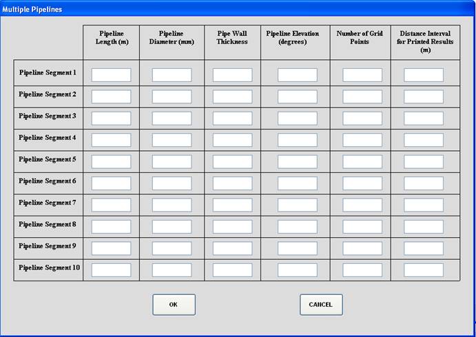
The Multiple Pipeline option allows the simulation of the failure of pipelines containing up to 10 pipeline segments. Similar to the single pipeline option (see 1.1), the user is required to input the pipe length, external diameter, wall thickness and elevation for each pipeline segment.
-
1.3 Pipeline Configuration: Heat Transfer Option – Pipeline Exposed to Air
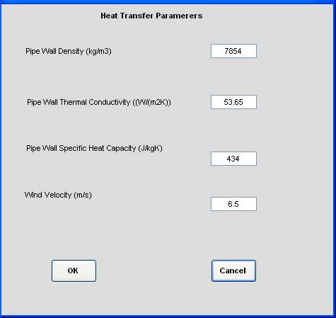
The Pipeline Exposed to Air heat transfer option requires material of construction data for the pipeline including its thermal conductivity and specific heat capacity as well as wind velocity. The default values used in PipeTech are for a carbon steel pipeline.
CONDITIONS
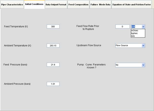
The initial steady state feed and ambient conditions prior to pipeline failure are the required inputs on this form. These include the feed temperature, pressure and the initial flow rate in either kg/s, m3/s or as a linear velocity (m/s) (see 2.1).

-
2.1 Feed Flow Rate Prior to Rupture
OUTPUT FORMAT
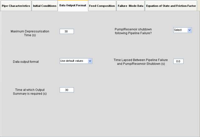
The maximum depressurisation time after pipeline failure to be simulated and the data output format (see 3.1) are user inputs on this form. In addition, depending on whether either a pump or reservoir is selected as the upstream flow source, the user will be prompted to supply the time duration which the pump or reservoir continues to operate post pipeline failure.
-
3.1 Time Interval Format
The maximum depressurisation time specified on the Data Output Format form (see 3) can be further broken up into 3 time intervals , the duration of the first and second time intervals can be set using this form. The user can also define the time increments used by PipeTech to present the output data in each of the 3 time intervals by adjusting the “Time Steps for Each Time Interval (s)”. The default values used in PipeTech for each time interval are: 0.1s for the First time interval, 0.2s for the Second time interval and 2s for the final time interval.
Numerical instabilities when simulating outflow are generally avoided by ensuring the Courant, Friedrichs and Lewy (CFL) condition which limits the maximum allowable discretisation time steps (Zucrow and Hoffman, 1976; Courant et al., 1952; Leveque, 2002) is satisfied. This is achieved in PipeTech by varying the CFL factor (Cf) in the range 0 < Cf ≤ 1. See Mahgerefteh et al. (2009) for further information about the CFL factor impact.

COMPOSITION
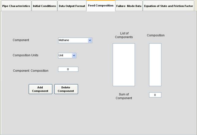
The Feed Composition can be input in either % mass or % mole. Any selected component can be removed from the “List of Components” by highlighting the component followed by pressing the “Delete Component” button.
MODE DATA
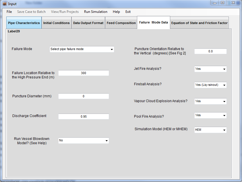
Failure Modes include full bore rupture, puncture along pipeline length and puncture across the pipe end circumference. The VB Model when activated will automatically check the applicability of the Vessel Blowdown model and if appropriate will perform simulations based on this model resulting in orders of magnitude reduction in the simulation run time.
OF STATE AND FRICTION FACTOR
RUN INPUT
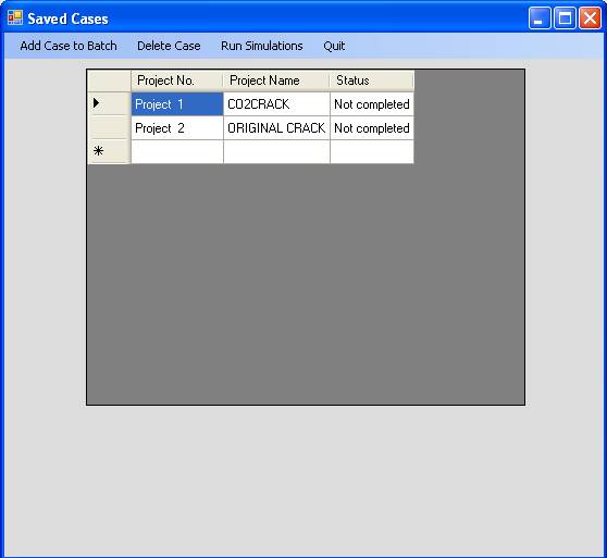
Either Single or Batch simulations may be performed. The latter allows automatic sequential simulations of up to 10 different failure scenarios (see 7.1). This option also allows re-run of previous cases hence reducing the time and effort required to setup and execute additional simulations where only changes in a small number of input parameters may be required.
-
7.1 Batch Run Simulation Status
OUTPUT RESULTS
RESULTS.XLS:
Upon Finish Command, output results are presented in 16 worksheets in a single Excel workbook which includes both graphical and tabular data. These worksheets are:
I. INPUT
A record of parameter values input to the simulation.
II. FIGURE 1: Pressure
Graph showing variation of discharge pressure at the failure point with time.
III. FIGURE 2: Discharge rate
Graph showing variation of discharge rate at the failure point with time.
IV. FIGURE 3: Cumulative Mass
Graph showing cumulative mass discharged with time.
V. FIGURE 4: Velocity
Graph showing the variation of discharge velocities at the failure point with time.
VI. FIGURE 5: Temperature
Graph showing the variation of discharge temperatures at the failure point with time.
VI. FIGURE 6: Density
Graph showing the variation of density at the failure point with time.
VI. FIGURE 7: Fireball Utility
Graph used to determine the maximum duration of a fireball.
VII. RUPTURE PLANE – Cum.Mass: Table showing variations over time of the:
• Total mass discharged since time zero (Total mass released [kg]),
• Liquid mass discharged since time zero (Mass of Liquid [kg]),
• Vapour mass discharged since time zero (Mass of Vapour [kg]),
• Individual component masses discharged since time zero [kg].
XI. RUPTURE DATA: Table showing variations over time of the:
• Mass discharge rate (Discharge Rate [kg/s]),
• Total mass discharged since time zero (Cumulative Mass [kg]),
• Discharge pressures at the failure point (Pexit1 and Pexit2 [bara]),
• Discharge temperatures at the failure point (Temp1 and Temp 2 [K]),
• Discharge densities at the failure point (Density 1 and Density 2 [kg/m3]),
• Discharge velocities at the failure point (Velocity 1 and Av. Velocity 2 [m/s]).
XII. RUPTURE PLANE – Vap.Mass: Table showing variations over time of the:
• Vapour mass discharged in the printed time interval (Mass of Vapour [kg]),
• Individual component mass fractions discharged in the printed time interval [kg].
XIV. RUPTURE PLANE – Liq.Mass: Table showing variations over time of the:
• Liquid mass discharged in the printed time interval (Mass of Liquid [kg]),
• Individual component mass fractions discharged in the printed time interval [kg].
XV. RUPTURE PLANE – Fluid Profile: Table showing variations over time, and at selected distances along the pipeline from the pump end, of the:
• Fluid temperature (T [K]),
• Fluid pressure (P [bara]),
• Fluid density (Rho [kg/m3]),
• Flow velocity (U [m/s]),
• Speed of sound through the fluid (A [m/s]),
• Specific enthalpy (Spcf- Enth [m2/s2]),
• Heat transfer coefficient (Heat Coff [W/m2.K]),
• Average pipe wall temperature (Av. Wall temp [K]),
• Phase index [ 1 = Liquid, 2 = Vapour, 3 = Two-phase].
XVI. STEADY STATE DATA: Table showing the initial steady state (time zero) values, at selected distances along the pipeline from the pump end, of the:
• Fluid temperature (Temp [K]),
• Fluid pressure (P [bara]),
• Fluid density (Rho [kg/m3]),
• Flow velocity (Vel [m/s])
• Speed of sound through the fluid (Spd-snd [m/s]),
• Phase index (Phase Index) [ 1 = Liquid, 2 = Vapour, 3 = Two-phase].
Additional data included are pipeline initial fluid inventory, the equivalent pressure, various temperatures through the wall of the pipeline, and the final fluid inventory in the pipeline at the end of the simulation.
XVII. FIREBALL UTILITY: Table showing the mass of inventory consumed in the fireball and radius of the fireball over time:
• Fireball Mass [kg],
• Radius [m]

